Essay
The Frozen Instrument
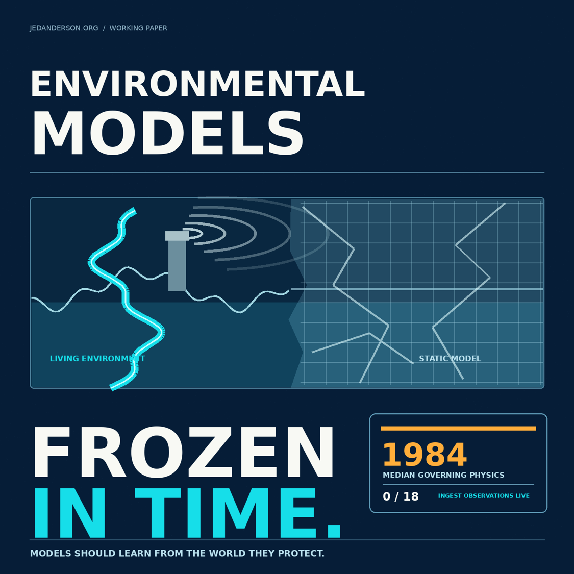
Environmental regulation runs on simulation models whose governing physics has a median age of 42 years, and not one of which learns from observation while it runs. This paper measures what that costs and derives, from first principles, why continuous modelling coupled to continuous sensing is the direction the field is compelled toward.
An inventory of 18 simulation models in routine use for United States permitting finds a median governing-formulation year of 1984, a median structural age of 42 years, and none that ingest observations while running. Decomposing the error of a regulatory prediction into physics, source parameters, and input freshness shows the physics term carries at most 12 percent of total error variance, so halving it removes 3 percent of total error while halving the parameter error removes 29 percent, implying a safety multiplier of about 9.2 under present practice that falls to 1.47 once the terms are measured away.
jedanderson.org corpus / working paper. September 2026.
Abstract. Environmental decisions in the United States are made with a small, stable set of simulation models: AERMOD for air dispersion, HSPF and SWAT for watersheds, WRAP for water availability, MODFLOW for groundwater, QUAL for stream oxygen, and roughly a dozen others. We inventory 18 of them and find a median governing-formulation year of 1984, a median structural age of 42 years, and that 0 of 18 ingest observations while running. We then decompose the error of a regulatory prediction into three independent terms: the physics of the model, the parameters describing the source, and the freshness of the inputs. Using the Guideline’s own stated uncertainty and EPA’s own emission-factor dispersion, the physics term carries 9 percent of total error variance when the model is run on climatological meteorology, and halving it removes 3 percent of total error; halving the parameter error removes 29 percent. The conclusion is structural rather than critical: model improvement has been concentrated on the smallest term in the budget, and the two larger terms cannot be reduced by any model, only by measurement. We show that the uncertainty implies a safety multiplier of about 9.2 under present practice, falling to 1.47 once the terms are measured away, a 6.3-fold recovery of operating headroom at unchanged risk; that a monthly-time-step allocation model passes months in which the daily target is violated on 12 days; and that a real change in a plant survives 1,176 times longer under annual verification than under hourly assimilation. The destination is not a better model but a different object: a persistent state estimator, coupled to sensing and to a pre-authorised action, running inside the sense-infer-decide-act loop rather than upstream of it.
1 · The models, and how old they are
Begin with the inventory rather than the complaint. Table 1 lists 18 simulation tools in routine use for permitting, planning and compliance in the United States, with the year the governing formulation was published and the year of the current software release.
| model | domain | formulation | governing basis | release | time step | input refresh |
|---|---|---|---|---|---|---|
| AERMOD / AERMET | air | 1991 | Gaussian plume (Sutton 1932; Pasquill–Gifford 1961) on Monin–Obukhov (1954) scaling | 2024 | 1 h steady state | 5-year met block |
| CTDMPLUS | air | 1987 | complex-terrain Gaussian | 2024 | 1 h steady state | 5-year met block |
| OCD | air | 1985 | overwater straight-line Gaussian | 2024 | 1 h steady state | 5-year met block |
| CMAQ | air | 1998 | Eulerian chemical transport | 2025 | minutes–hours | episode, offline |
| MOVES | air | 1978 | MOBILE emission-factor lineage | 2023 | aggregated | periodic |
| HSPF | water | 1966 | Stanford Watershed Model IV moisture accounting | 2020 | 1 h | historic record |
| SWMM | water | 1971 | kinematic-wave urban runoff | 2022 | minutes–hours | design storm |
| QUAL2K | water | 1925 | Streeter–Phelps oxygen sag; QUAL lineage from about 1970 | 2018 | steady / diel | critical condition |
| WASP | water | 1983 | compartmental mass balance | 2021 | variable | historic record |
| SWAT | water | 1993 | curve number plus crop routines | 2023 | 1 day | historic record |
| WRAP / TCEQ WAM | water | 1988 | prior appropriation on naturalised monthly flows | 2024 | 1 month | 1940s–1990s hydrology |
| HEC-RAS | water | 1968 | HEC-2 step backwater; 1-D St Venant | 2024 | steady / unsteady | design flood |
| TR-55 curve number | water | 1954 | SCS curve number | 1986 | event | design storm |
| MODFLOW | groundwater | 1984 | block-centred finite-difference flow | 2024 | stress period | calibration epoch |
| EPANET | water | 1993 | network hydraulics with first-order decay | 2020 | variable | design demand |
| Johnson–Ettinger | soil gas | 1991 | 1-D steady vapour intrusion | 2017 | steady state | one-time |
| 7Q10 low flow | water | 1960 | stationary low-flow order statistic | 1960 | static | gauge epoch |
Table 1. Formulation years are the publication of the governing physics or method, not of the software. Release years are the most recent public version. The full inventory behind the statistics lists AERMET separately, giving 18 entries.
The statistics are the point. Median formulation year 1984; median structural age 42 years; 67 percent of the formulations predate 1990. Median release year 2023, a code age of 3 years. The gap between those two numbers, roughly four decades, is the distance between how current these tools appear and how current their physics is.
Software releases have been frequent. The epoch of the physics has not moved.
VERIFIED AGAINST PRIMARY SOURCES
This is not an accusation of negligence. AERMOD’s 2024 revision was real work: mobile-source treatment near roadways, a new tier-3 method for converting nitrogen oxides to nitrogen dioxide, and a marine boundary-layer algorithm for overwater sources. But the object being revised remains what the Guideline itself calls it, a steady-state Gaussian plume model: each hour is solved as if the atmosphere were uniform, stationary and straight-line for that hour, then discarded. The same holds across the table. WRAP allocates water rights on a monthly time step against naturalised flows whose record, for most Texas basins, ends in the 1990s. QUAL descends from a 1925 oxygen-sag equation. TR-55 curve numbers were fitted to agricultural plots in the 1950s.
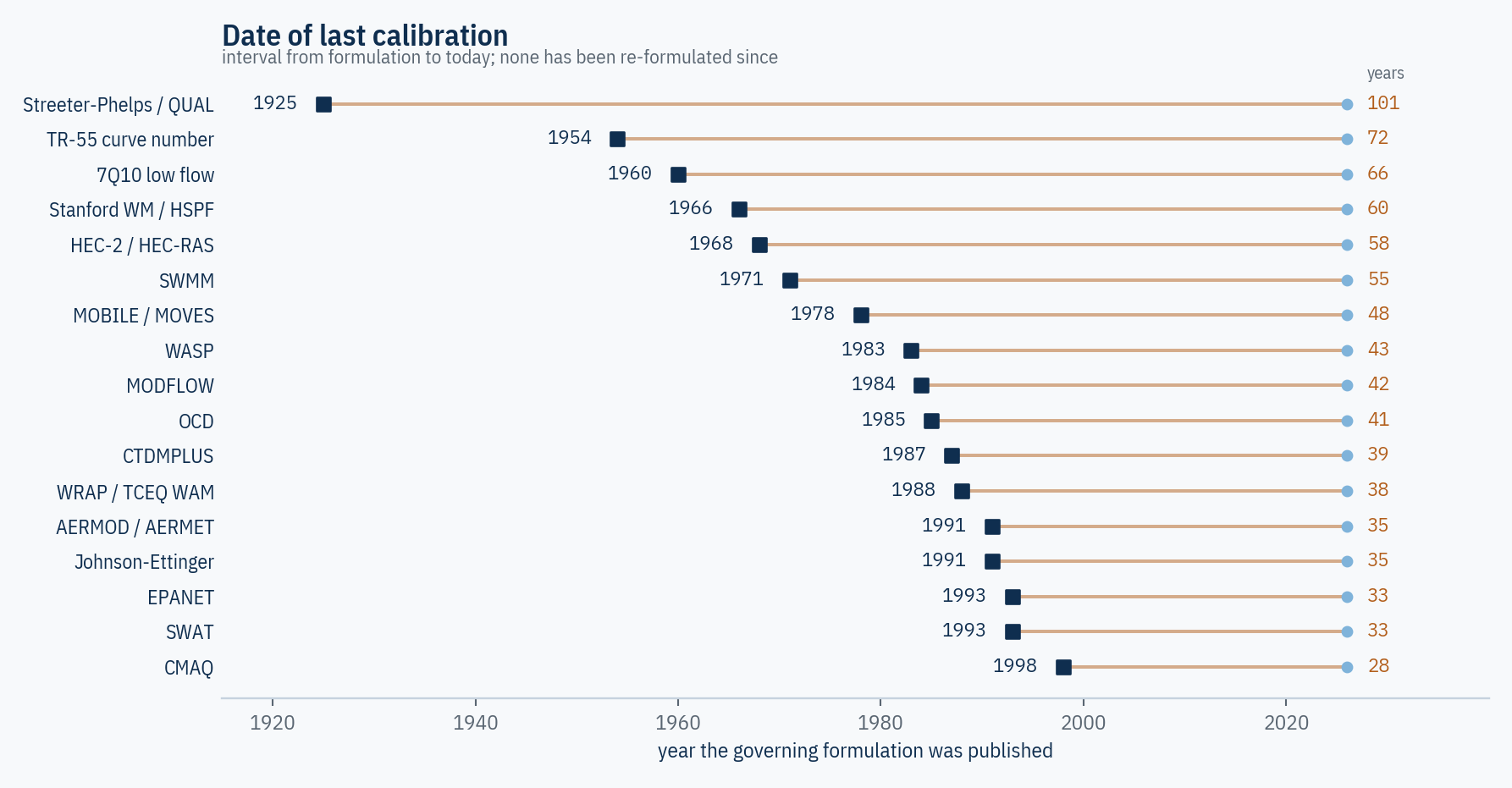
Figure 1. Publication year of the governing formulation for each tool and the interval to the present. Almost the entire regulatory modelling stack was written between 1925 and 1998.
2 · The three assumptions that date them
Age alone proves nothing; Newtonian mechanics is older still and works. What matters is whether the assumptions that made these formulations tractable in their decade are the assumptions that limit them now. Three recur across the table, and each was a response to a constraint that has since lifted.
Steady state, because integration was expensive. A steady-state solution replaces a differential equation in time with an algebraic one. AERMOD solves each hour as an independent equilibrium; Johnson–Ettinger solves a vapour intrusion problem with no time coordinate at all; QUAL’s classical use is a critical-condition steady solution. This was the correct engineering choice when a model run was a capital event. Its cost is that transients, the very events environmental protection exists for, are represented as sequences of equilibria that the model never connects.
Stationarity, because the record was the only source of futures. The 7Q10 low flow, the design storm, the five-year meteorological block and the WAM period of record all assume that a fixed historical sample is an unbiased description of the future. That assumption was defensible when the alternative was nothing. It is now the weakest link in every water model: a naturalised flow record ending in the 1990s does not contain the 2010–2015 Texas drought, and a model built on it will report availability that the basin has since demonstrated it does not have.
Open loop, because measurement was scarce, and then because the rules required it. The third assumption is the one worth dwelling on, because it is not merely inherited. It is written down. The Guideline on Air Quality Models, discussing the comparison of modelled against observed concentrations, states that because of the uncertainty in paired modelled and observed values, attempts at calibration of models based on those comparisons are of questionable benefit and shall not be done.
The regulatory framework does not simply omit the step in which a model learns from the receptor it is predicting. It forecloses it.
VERIFIED: 40 CFR 51 APP. W · THE CONTROL READING IS OURS
The stated reason is sound on its own terms: concentrations paired in time and space are noisy, and tuning a model to noise produces a worse model. But the consequence, read in control terms, is that the loop between prediction and observation is severed by rule. A model that may not be corrected by what is measured downwind of it is, by construction, an open-loop element. Every result in the rest of this paper follows from that severance.
3 · Where the error actually is
The dispersion physics is the smallest of the three error terms, and the only one a better model can fix.
A regulatory concentration estimate is a product: an emission rate, a dispersion factor determined by meteorology, and the model’s representation of the physics. In logarithms a product becomes a sum, so the errors add in variance, and we can ask which term dominates. We take each term’s magnitude from the regulatory record itself rather than assuming it.
The structural term comes from the Guideline’s own uncertainty discussion, which puts the irreducible uncertainty of Gaussian plume models at about ±50 percent, and notes that wind-direction errors of five to ten degrees can produce concentration errors of 20 to 70 percent at a particular time and place. Read as a lognormal spread, ±50 percent is a log standard deviation of 0.41.
The parameter term comes from emission factors. EPA’s own compendium concedes that roughly half the sources in a category emit more than the factor says, and does not publish the dispersion. At a geometric standard deviation of three, a value consistent with the factor-of-five-to-seven and order-of-magnitude inventory errors measured in Houston, the log standard deviation is 1.10.
The input term is what a model forfeits by being run on typical rather than actual conditions. Computed directly from a Gaussian plume over 400,000 synthetic hours at a 50 m effective stack height, the hour-to-hour spread of the dispersion factor has a log standard deviation of 0.67. Run on climatology, all of it becomes error; run on live meteorology, none of it does; in between it decays with the age of the input.
| input age | source | weather | physics | sigma |
|---|---|---|---|---|
| live | 88 | 0 | 12 | 1.17 |
| 1 hour | 87 | 1 | 12 | 1.18 |
| 1 day | 76 | 14 | 10 | 1.26 |
| 3 days | 69 | 22 | 9 | 1.33 |
| 1 month | 66 | 25 | 9 | 1.35 |
| climatology | 66 | 25 | 9 | 1.35 |
Table 2. Error budget as a share of total variance, against the age of the meteorological input. First three columns are percent of variance.
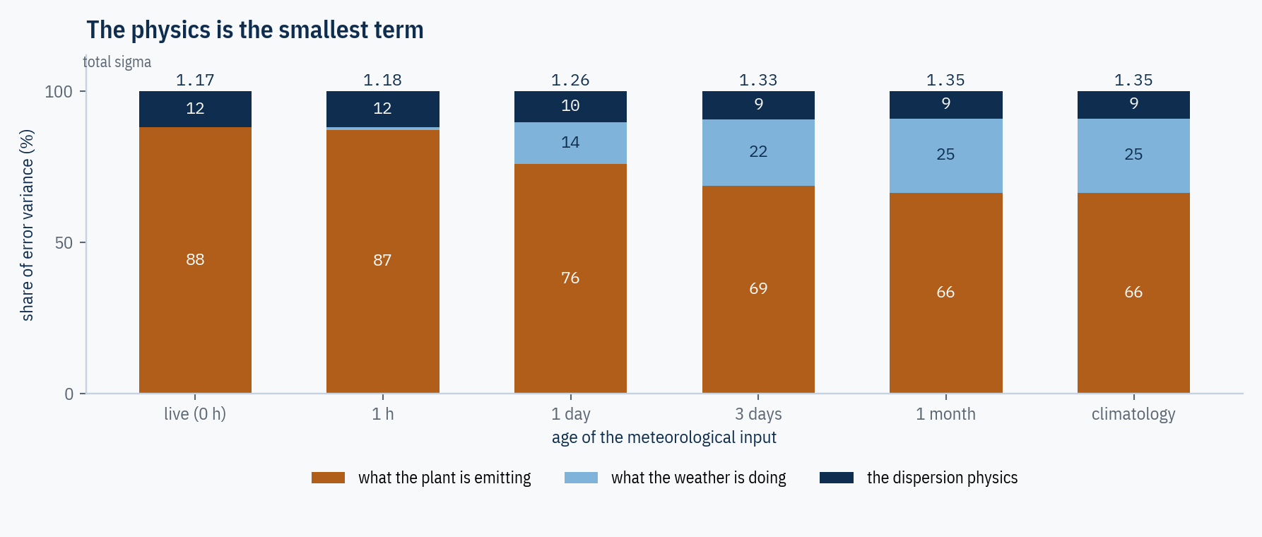
Figure 2. Composition of total error variance against the age of the meteorological input. The physics term never exceeds 12 percent of the budget in any regime.
Now the operational question. Suppose you could halve one term. Which?
| input regime | physics | source | weather |
|---|---|---|---|
| live inputs | 5 | 42 | 0 |
| day-old | 4 | 34 | 5 |
| climatology | 3 | 29 | 10 |
Table 3. Reduction in total predictive error from halving one error term, by input regime, in percent.
Thirty-five years of dispersion-model development, conducted carefully and in good faith, has been spent on the term worth three to five percent. This is not an argument that the work was wasted; the physics term is the only one a modeller controls, so it is the only one a modelling programme can address. It is an argument that the binding constraint was never in the model. The parameter term is fixed by metering the source. The input term is fixed by feeding the model live weather. Neither is a modelling problem, and both are now cheap.
Computed from stated regulatory uncertainties. Emission-factor spread assumed.
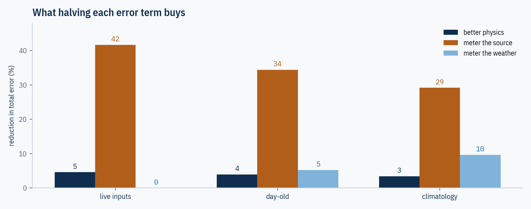
Figure 3. What each class of improvement buys, in reduction of total predictive error, under three input regimes.
4 · What the error budget costs
A margin is not caution. It is the price of the error budget, paid every hour.
Uncertainty has to be absorbed somewhere, and in permitting it is absorbed by conservatism: worst-case stacking, upper-bound emission factors, the worst modelled hour. If the model’s output were treated as an unbiased central estimate, the multiplier required to keep the true value below the limit with 95 percent confidence is exp(1.645 sigma). Under present practice that is about 9.2. Measure the source and it falls to 3.96. Add live meteorology and it falls to 2.34. Add continuous emissions monitoring and receptor assimilation and it reaches 1.47.
We are careful about what this is. It is not a claim that permits contain a stated ninefold factor. It is the size of the conservatism the uncertainty requires, and the regulatory system supplies it implicitly, through the convention of stacking worst cases rather than through a published number. The practical reading is the ratio: each error term measured away returns roughly its share of the margin as operating headroom, at unchanged risk to the receptor.
Computed. Margins implied, not stated in any permit.
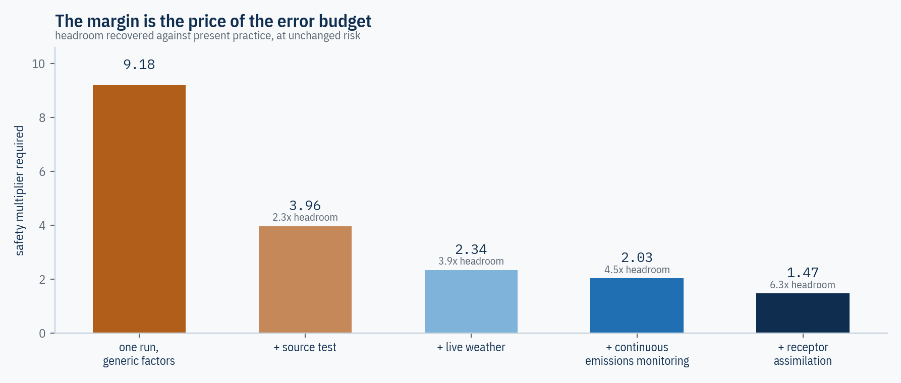
Figure 4. Safety multiplier implied by the error budget under successive measurement regimes, and the headroom recovered relative to present practice.
5 · The time step is a filter, not an approximation
A monthly model of a daily world is not a coarse view of it. It is blind to a class of event by construction.
The Texas water availability models allocate on a monthly time step. The intuition that a monthly model is a slightly blurred daily model is wrong, and the error is one of kind. Averaging is a low-pass filter: variance below the sampling period is not attenuated, it is removed, and events shorter than the step cannot appear in the output at any magnitude.
We generated daily flows as a lognormal autoregressive process and asked how often a month passes a monthly-mean test while containing days below the same threshold. At a daily coefficient of variation of 1.2 and a target of 0.7 of mean flow, 65 percent of months pass the monthly test, and of those passing months 99 percent contain at least one day below target, averaging 12 short days per compliant month.
The events the monthly model cannot represent are exactly the low-flow days that instream flow requirements exist to prevent. This is the same result the corpus reached for air from the sampling theorem, arriving from the other direction: the aliasing is not noise, it is a confident and internally consistent account of a different river.
| daily CV | target | months passing (%) | of those, with short days (%) | short days per month |
|---|---|---|---|---|
| 0.8 | 0.5 | 89 | 79 | 6.2 |
| 0.8 | 0.7 | 69 | 92 | 8.6 |
| 1.2 | 0.5 | 83 | 95 | 9.6 |
| 1.2 | 0.7 | 65 | 99 | 11.9 |
| 1.8 | 0.5 | 76 | 100 | 12.8 |
| 1.8 | 0.7 | 57 | 100 | 14.6 |
Table 4. What a monthly time step conceals. Of the months that pass a monthly-mean test, the share that still contain days below the same target, and how many such days.
Simulation. Synthetic flow statistics.
6 · What a continuous model would actually buy
Cadence compounds. Accuracy does not.
The clearest operational case for continuity is not accuracy but detection. Let a control device degrade so that true emissions step up and stay up, and let the model be told nothing. Each regime learns about it only through whatever observation it is checked against. Holding the false-alarm budget fixed at one per ten years across all regimes, and applying the optimal sequential test, the results are in Table 5.
| verification regime | 30% loss of control (days) | doubling (days) |
|---|---|---|
| annual stack test | 888.3 | 395.54 |
| semiannual report | 669.2 | 211.76 |
| quarterly monitoring | 387.5 | 113.69 |
| monthly | 173.5 | 44.67 |
| weekly | 63.0 | 13.00 |
| daily residual | 12.3 | 2.38 |
| hourly assimilation | 0.8 | 0.13 |
Table 5. Mean time a real change survives undetected, at a fixed false-alarm budget of one per ten years. Delays at the three slowest cadences are censored at the simulation horizon and are therefore lower bounds.
Then the comparison that decides where to spend. A better model reduces the noise on the model-versus-observation residual; a faster cadence reduces the interval between residuals. Starting from quarterly verification, halving the residual noise, which is a very good decade of model development, cuts detection delay by 63 percent. Simply moving from quarterly to monthly, with the same model, cuts it by 58 percent. The reason is structural: detection delay is approximately the logarithm of the certainty you demand divided by the information you receive per unit time. Halving the noise buys a fixed factor once. Halving the interval buys a comparable factor and keeps buying it every time you halve again.
Agrees with Lorden scaling. Slow cadences are censored lower bounds.
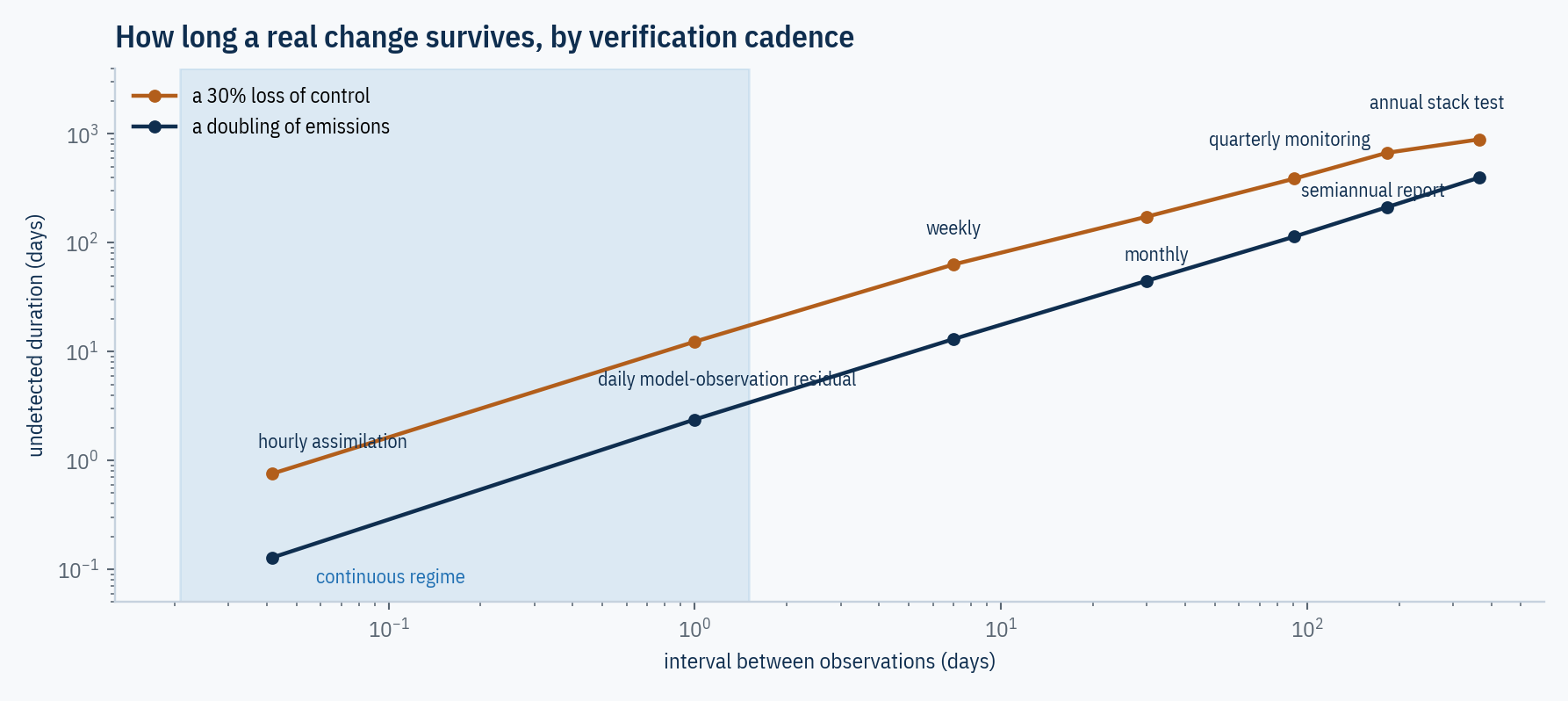
Figure 5. Time a real change in the plant survives undetected against the interval between observations, at a fixed false-alarm budget of one per ten years. Slopes are near unity on log axes: delay is proportional to cadence.
7 · Where modelling is going, and why it has to
Three developments have removed the constraints that justified the frozen instrument, and they arrived within roughly five years of each other.
The cost of a model run collapsed. Foundation models trained on the planet’s record now do in seconds what physics simulation did in hours. Aurora, trained on more than a million hours of geophysical data, matches or beats the operational CAMS system on 74 percent of air-quality targets across lead times and 89 percent at a three-day lead, and beats the operational IFS on 92 percent of targets while running roughly 5,000 times faster. When a run stops being a project and becomes an operation you can afford hourly, the economic argument for a one-time run disappears.
Models became differentiable, so they can learn without being abandoned. The choice that framed the last decade, mechanistic model versus machine learning, has been dissolved by differentiable modelling: physical structure retained, with neural components embedded inside it and gradients computed through the whole, so parameters and unknown relationships are learned end-to-end from data. Under data-scarce conditions these hybrids have outperformed pure learning on short-term dynamics and decadal trends, because the physics constrains them. This matters for regulation specifically: a differentiable AERMOD would keep the conservation laws and the boundary-layer scaling that make it defensible, and gain the ability to be corrected by the fenceline instead of being frozen against it.
Assimilation became the organising idea, at planetary scale. Destination Earth, the European Union’s Earth-system digital twin programme, has moved from development into operation: a weather-induced extremes twin combining a continuous global component at kilometre scale with an on-demand regional component, and a climate adaptation twin producing multi-decadal kilometre-scale simulations with hourly output. Its third phase runs 2026 to 2028. Whatever one thinks of the branding, the architecture is the argument: a model that runs continuously, ingests observations continuously, and is queried rather than commissioned.
Nature 2025; Nature Reviews Earth & Environment 2023; ECMWF.
The first-principles reason this is not a fashion
Strip the technology away and the direction survives, because four independent results all point the same way, and none of them is about computers.
Conant and Ashby. Every good regulator of a system must contain a model of that system. The theorem is often quoted to justify modelling. It also constrains it: the regulator’s model must be a model of the system’s present state, and a model of a state that has moved is a model of a different system.
The degradation theorem. A model calibrated once holds information about the plant that decays monotonically as the plant drifts, cannot be restored by any reprocessing of the model, and leaves an uncertainty that grows without bound. A frozen model has a half-life; an assimilating one has a steady state.
The sampling theorem. A model whose inputs are refreshed more slowly than the world changes does not produce a blurred picture of that world; it produces a confident picture of a different one. This is the monthly WAM result in section 5 and the five-year meteorological block in section 3.
The bandwidth limit. A loop cannot reject a disturbance faster than its own bandwidth, and the bandwidth of a loop with delay is capped near its reciprocal. A model that participates in protection at all participates as an element of that loop, and its cadence is part of the loop’s delay.
Together these say something stronger than that continuous would be nicer. They say that a model used for control must be a state estimator, that a state estimator must be corrected by observation, and that its correction interval must be shorter than the timescale of what it estimates. Anything else is not a worse controller. It is not a controller.
8 · What the next instrument looks like
The destination is not a faster AERMOD. It is a different object with a different job description, and it can be specified now.
It runs, rather than being run. A persistent process with a current state and an uncertainty attached to it, not a study that is commissioned, executed and archived. The deliverable stops being a report and becomes an endpoint that can be asked what the receptor concentration is right now and how confident it is.
It keeps the physics and surrenders the freeze. Conservation of mass and energy, boundary-layer scaling, oxygen-sag kinetics: these carry the reach that lets a model be right about conditions it has never seen, which is why the corpus’s own reach experiment found pattern learners missing every hypoxic outcome outside their record while the explanation missed none. Learned components run inside that envelope as accelerators and as correctors, and the system must detect its own departure from the record rather than answering confidently off the edge of it.
It assimilates, which requires a rule change. The prohibition on calibrating models against paired observations was a reasonable response to noisy paired comparisons. Modern data assimilation is not calibration to a paired comparison; it is a filter that weights observation against prediction by their respective uncertainties and is mathematically incapable of chasing noise it has correctly characterised. The reform is narrow and stateable: permit assimilation under a published error model, with the filter, its innovations and its uncertainty on the record and contestable.
It closes on the variable that carries the harm. Exposure at a receptor rather than tons at a stack; oxygen at the sag rather than load at the outfall; days below the instream target rather than the monthly mean. The corpus has documented what happens when a loop is closed automatically on a scalar aggregate: the aggregate is optimised and the spatial structure of harm is not.
Its output is a function, not a number. A continuously running estimator naturally produces an envelope, a rule evaluated against the measured state, rather than a scalar limit good for five years. That is where this paper meets the rest of the corpus, and it is why the modelling question and the permitting question are the same question.
9 · The instrument was never the problem. Its coupling was.
The models environmental professionals use are not bad models. They are good models of their decade, executing an architecture that was correct when measurement was scarce and computation was expensive: predict once, conservatively, then act on the prediction. Our inventory finds a median structural age of 42 years and no instance of a regulatory model that learns from observation while it runs. Our error decomposition finds that the physics those models encode is the smallest term in the budget, worth 3 percent of total error if halved, while the two larger terms yield only to measurement. Our detection analysis finds cadence beating accuracy, and continuing to beat it at every doubling.
So the answer to whether the models should themselves be continuous is yes, but the reason is not that continuous is modern. It is that a model used inside a protection loop is a state estimator, and a state estimator that is not corrected is not an estimator of the present. Everything in the technology trend, cheap inference, differentiable physics, operational digital twins, is the removal of an excuse. The remaining obstacles are a sentence in Appendix W, a monthly time step in a water availability model, a five-year block of meteorology, and the habit of treating a prediction as a fact.
We do not need a better model of the plant. We need a model that is still looking at it.
Methods
All computations were written and executed for this paper in Python (NumPy, SciPy) and accompany it with run logs.
Inventory, §1. Formulation years are the publication of the governing physics or method; release years are the latest public version. Statistics are unweighted across 18 entries.
Error budget, §3. Errors are treated as independent lognormal factors, so log-variances add. The structural term is Appendix W’s stated ±50 percent irreducible uncertainty read as a lognormal one-sigma. The parameter term uses a geometric standard deviation of 3 for facility-to-facility emission-factor dispersion; this is a modelling assumption, since EPA does not publish the dispersion. The input term is computed from a Gaussian plume with Briggs open-country coefficients at 50 m effective stack height over 400,000 synthetic hours, with a Weibull wind (shape 2, mean 4 m/s) truncated below 1 m/s by rejection sampling and an illustrative stability-class distribution; input staleness decays the term through an Ornstein–Uhlenbeck correlation with a 72-hour timescale.
Margin, §4. exp(1.645·sigma) for a 95 percent one-sided bound on a lognormal error. Aliasing, §5. Daily flows as a lognormal AR(1) process, 200 years, aggregated into 30-day blocks. Detection, §6. CUSUM on log-residuals with thresholds calibrated by simulation to a 3,650-day mean false-alarm run length in every regime, cross-checked against the Lorden/Siegmund asymptotic delay ln(ARL)/KL; agreement is within 10 to 15 percent where the delay exceeds a few samples.
Limitations. The plume is a screening calculation, not AERMOD, and uses synthetic meteorology; only ratios and shares should be quoted from it. The emission-factor dispersion is assumed, and the error budget’s headline shares move with it: at a geometric standard deviation of 2 rather than 3 the parameter share falls substantially, though it remains the largest term. The margin figures are the conservatism the uncertainty implies, not a factor stated in any permit. The detection delays at annual, semiannual and quarterly cadence are censored at the simulation horizon and are therefore lower bounds; the true delays are longer, which strengthens rather than weakens the finding. Formulation years for a few entries mark a lineage rather than a single paper, and reasonable people would date QUAL from 1970 rather than from Streeter and Phelps in 1925; the median moves by about two years either way. Nothing here was validated against an operational model run or a real facility, and the obvious next step is to repeat the error decomposition against a real AERMOD analysis with a fenceline record, which would convert several assumptions into measurements.
Principal sources. 40 C.F.R. part 51, appendix W (Guideline on Air Quality Models), including its uncertainty discussion and the provision that model calibration against paired observations shall not be done; final revisions published 89 Fed. Reg. (Nov. 29, 2024), effective January 28, 2025, with AERMOD version 24142. EPA Office of Inspector General 18-P-0241 (Sept. 5, 2018) for the 1978 promulgation of appendix W and AERMOD’s 2005 designation. EPA SCRAM, preferred and recommended models. Wurbs, WRAP modelling system reference and fundamentals manuals, and TCEQ Water Availability Modeling System documentation. Burges and Crawford on the Stanford Watershed Model (1959–1966) and its descent to HSPF. Bodnar et al., A foundation model for the Earth system, Nature 641:1180–1187 (2025). Shen et al., Differentiable modelling to unify machine learning and physical models for geosciences, Nature Reviews Earth & Environment 4:552–567 (2023). ECMWF and ESA, Destination Earth programme documentation and the confirmation of phase three (June 2026 to June 2028). Conant and Ashby, Every good regulator of a system must be a model of that system, International Journal of Systems Science 1:89–97 (1970). Lorden (1971) and Siegmund (1985) for sequential change detection. Standard model lineages (Streeter and Phelps 1925; SCS curve number 1954; Monin and Obukhov 1954; Pasquill 1961 and Gifford 1961; Briggs 1973; MODFLOW 1984) are given as historical background.
Related: The End of the Snapshot
Licensed CC-BY-4.0 .
Markdown source: https://jedanderson.org/essays/frozen-instrument.md
Source on GitHub: /src/content/essays/frozen-instrument.md
Cite this
@misc{anderson_2026_frozen_instrument,
  author = {Jed Anderson},
  title  = {The Frozen Instrument},
  year   = {2026},
  url    = {https://jedanderson.org/essays/frozen-instrument},
  note   = {Accessed: 2026-09-15}
} Anderson, J. (2026). The Frozen Instrument. Retrieved from https://jedanderson.org/essays/frozen-instrument
Anderson, Jed. "The Frozen Instrument." Jed Anderson, September 9, 2026, https://jedanderson.org/essays/frozen-instrument.