The End of the Snapshot

Environmental protection has been steered by pictures: models run once, on chosen inputs, whose outputs became facts for a decade. Seven properties of any one-time model, computed rather than asserted, and what replaces it.

Environmental permits are written from models run once, on chosen inputs, whose outputs become legal facts for five to fifteen years. Seven properties of any one-time model are derived and simulated here: averaging the inputs is not averaging the answer, a design value is one draw from an unreported sampling distribution, stacked maxima are blind to coincidence, a short test of an intermittent source fails to identify a number at all, every frozen model has a half-life, the value of a model is the age of its inputs, and the resulting conservatism has been paid in production every hour for fifty years. The conclusion is not that models are bad but that a model is a state estimator that was mistakenly used as an oracle.

September 2026. Sense → infer → decide → act. Code and run logs accompany this piece.

Almost everything we know about a regulated facility’s effect on the world comes from a model that was run once. Five years of hourly weather, a critical low flow, an assumed emission rate, a grid of receptors: one run, one number, and then that number is the legal truth about the place until the permit is renewed. The corpus has treated this as a latency problem, and it is one. But there is a separate set of errors that belong to the snapshot as such, and they do not go away by running the snapshot sooner or more carefully.

This piece computes them. Each section states a property of one-time modelling, derives it, tests it numerically, and tags how far to trust it: VERIFIED where a derivation and a simulation agree, ESTIMATE or PROBABLE for an inference or an order of magnitude. The claim at the end is not that models are bad. It is that a model is a state estimator that was mistakenly used as an oracle, and that the machinery to run it as a state estimator now exists and is cheaper than the margin it replaces.

01 · A snapshot is a model run once, whose output becomes a fact.

It was not a mistake. It was the correct engineering answer to a measurement budget, and the budget has changed.

Here is the practice, stated plainly. An engineer builds a model of a facility and its receiving environment. The model is run on a chosen set of inputs: an assumed emission rate, five years of hourly weather from a nearby airport, a critical low-flow statistic for a river, a design storm. It produces a number. The number goes into a permit, and for the next five to fifteen years that number is treated as a fact about the world, unexamined, whatever the facility or the atmosphere or the river subsequently does.

This corpus has called that an open-loop controller, and it has also made a correction worth repeating, because it disciplines everything that follows. Under a hard measurement constraint, feedforward with a conservative model and a safety factor is not a failure of nerve. It is the correct engineering choice. Congress wrote the constraint into the statute itself, permitting alternatives to continuous monitoring where they provide sufficiently reliable and timely information. The snapshot was never a description of reality. It was a rationing of scarce verification, and it bit hard.

So the case for the end of the snapshot cannot be that it was foolish. It has to be one of two things: that the snapshot has errors which no amount of care inside the snapshot can remove, and that the constraint which justified it has lifted. Both are true, and the first is more interesting than the second. What follows are seven properties of any one-time model. None of them is a modelling mistake. Each is a consequence of taking one picture of something that moves.

The object under discussion. A PSD dispersion analysis: five years of hourly meteorology, receptors on a grid, the worst modelled hour converted into a static pounds-per-hour limit. An NPDES analysis: a critical low-flow statistic (7Q10) and a critical temperature, converted into a fixed effluent limit. Both are steering by picture.

FRAMING

02 · Averaging the inputs is not averaging the answer.

A single run at representative conditions understates the mean whenever the response is curved, and the error has a sign.

Ground-level concentration from a stack is inversely proportional to wind speed. Inverse is a convex function, and for convex functions the average of the answers is larger than the answer at the average input. That is Jensen’s inequality, and here it has a closed form. If hourly wind follows a Weibull distribution of shape k, the ratio of the true mean concentration to the concentration computed at the mean wind is exactly Gamma(1 − 1/k) × Gamma(1 + 1/k). For a Rayleigh wind, k = 2, the ratio is exactly π/2: modelling at the mean wind understates the mean by 57 percent.

The obvious objection is that models refuse to run at calm winds, which truncates the very tail that drives the identity. It does, and the effect survives it. Truncating the wind distribution below 1 m/s still leaves a 30 percent understatement; below 2 m/s, 16 percent. Adding stability variation on top, across 600,000 synthetic hours at a 50-metre stack, the mean of the hourly answers is 1.30 times the single answer computed at mean conditions.

Two things follow, and the second is the one that matters. First, the error is directional, not random: a conservative modeller cannot pad against it without knowing its size, and the size depends on the variance of the input, which the snapshot does not carry. Second, and generally, the snapshot commits an error of a specific kind. It evaluates f at a summary of the inputs when the quantity of interest is a summary of f over the inputs. Every environmental response that matters is curved. Dose-response has thresholds. Ozone chemistry is nonlinear in its precursors. Reaeration goes as the square root of velocity over depth to the three-halves. Wherever there is curvature, the picture of the average is not the average of the pictures, and no care taken inside the single run repairs it.

Exact. E[1/u] ÷ (1/E[u]) = Γ(1−1/k)·Γ(1+1/k): k = 1.5 → 2.42; k = 2 → π/2 = 1.571; k = 2.5 → 1.32; k = 3 → 1.21. With a low-wind cutoff (rejection sampling, mean wind 4 m/s): 0.5 m/s → 1.41; 1.0 → 1.30; 1.5 → 1.22; 2.0 → 1.16. Wind and stability together (600,000 hours, 50 m effective height, Briggs open-country coefficients): mean of the hourly answers ÷ one run at mean inputs = 1.30; 99th percentile hour = 3.6× the mean hour.

VERIFIED: DERIVED AND SIMULATED

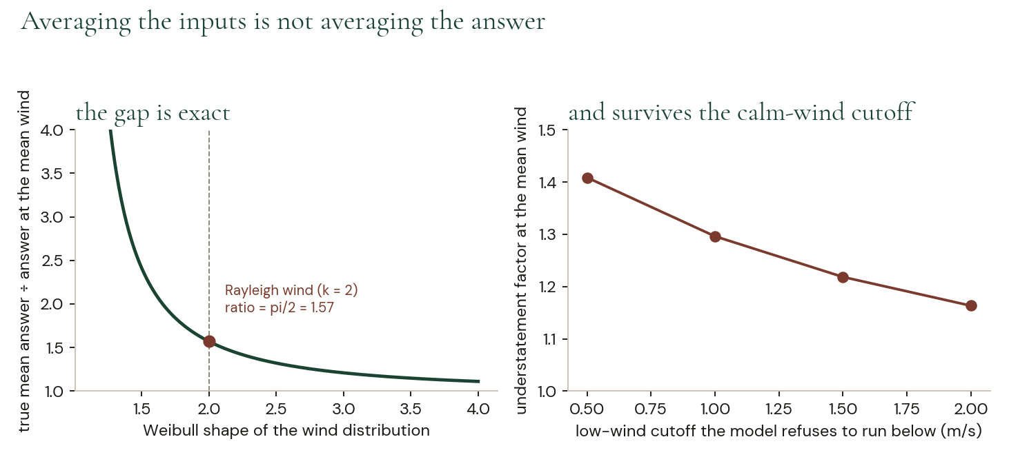
Figure 1. Left: the exact ratio between the true mean concentration and the concentration at the mean wind, as a function of the wind distribution’s shape. Right: the same gap after the low-wind cutoff that real models impose.

03 · A design value is one draw from a distribution nobody reports.

The number in the permit has a sampling error, it is computable, and it is often larger than the compliance margin it is compared against.

Take the practice at its own word. Five years of hourly meteorology is a sample. Run the model over it and rank the results, and the design value is an order statistic of that sample: the highest hour, or the eighth-highest, or a high percentile. Order statistics have sampling distributions. Hourly air-quality maxima sit in the Gumbel domain of attraction, which is to say they have an approximately exponential upper tail of some scale, and for such a tail the sampling standard deviation of the k-th largest of many draws is known in closed form: about 1.28 tail-scales for the single maximum, 0.37 for the eighth-highest, 0.20 for the twenty-sixth. Simulation over 1,500 independent five-year records reproduces both to within one percent.

Put that in permit units. A plant whose eighth-highest hour comes out at 80 percent of the standard, with an hourly tail scale of 15 percent of that design value, has a sampling standard deviation of 5.5 percent of the design value and a 90 percent band running from 0.91 to 1.09 times the number written down. Had the rule used the highest hour instead, the standard deviation would be 19 percent. Identical physics, identical plant, a different five years, a materially different permit.

Notice what that says about the rules themselves. The regulatory preference for the eighth-highest hour over the highest is already an admission that a single draw is unstable; it buys a 3.5-fold reduction in sampling error, and says so nowhere. The residual is carried nowhere either. A design value is reported as a scalar, compared against a standard as a scalar, and defended in a hearing as a scalar, when it is an estimate with a standard error that the same model run could have produced for free.

And the sample is not just noisy, it is short. For an exponential tail the expected maximum grows with the logarithm of the record length. A permit modelled on five years and operated for fifteen faces an expected maximum about 1.1 tail-scales higher than the one it was designed against, roughly 10 percent, from the same plant and the same physics, with nothing changed but how long the exposure has to run.

Sampling SD of the k-th largest (exponential tail, in tail-scales): 1st 1.283, 2nd 0.803, 4th 0.533, 8th 0.365, 26th 0.198. Simulated over 1,500 five-year records: 1st 1.267, 8th 0.368. Permit units (8th-high at 80% of the standard, tail scale 15% of it): SD 5.5% of the design value, 90% band 0.91×–1.09×; single highest hour, SD 19.2%, 3.5× wider. Record length: expected maximum grows as β·ln(N); 5 years → 11.26 β, 15 years → 12.36 β.

VERIFIED: THEORY AND SIMULATION AGREE

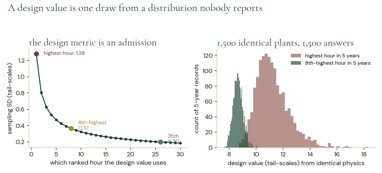
Figure 2. Left: sampling error of the design value against which ranked hour the rule selects. Right: 1,500 identical plants modelled on 1,500 different five-year records, and the answers they get.

The snapshot holds one number from each margin and multiplies them. A receptor experiences a joint distribution.

The conservative habit in one-time modelling is to stack worst cases: the maximum permitted emission rate on the worst modelled hour, the design storm on the saturated catchment, the critical low flow on the critical temperature. This is defended as protective, and as a bound on the product it is. But a bound on the product is not a statement about how often the two factors are large together, and it is the joint frequency that a person downwind actually experiences.

The experiment holds the plant and the design number fixed and varies only the correlation between high emissions and poor dispersion. At zero correlation, essentially no hours exceed the design number. At a correlation of 0.4, one to two hours a year. At 0.8, close to six. The 99.9th-percentile hour rises by nearly a factor of three across the same range. Nothing about the facility changed. Nothing about the model’s inputs changed in their margins. Only the coupling changed, and the snapshot has no place to record a coupling: it is a scalar produced by multiplying two scalars.

The correlations in question are not exotic. Hot stagnant afternoons raise cooling demand, raise throughput, and suppress dispersion at the same time. Winter inversions coincide with heating load. Startups and shutdowns cluster around the weather events that caused them. Drought lowers river flow, raises water temperature, lowers oxygen saturation, and concentrates the discharge, all at once, which is exactly the compound case the corpus found the learned models missing in the Streeter-Phelps experiment. Conservatism in each margin does not buy conservatism in the joint tail, and the snapshot cannot tell you which you have.

Design number = short-term emission cap at the 99th percentile × worst modelled hour (99.99th percentile of dispersion) = 6.26e-04. Hours per year above it, plant and design number unchanged: correlation 0.0 → 0.0 h; 0.2 → 0.5 h; 0.4 → 1.2 h; 0.6 → 2.9 h; 0.8 → 5.8 h. 99.9th percentile hour rises from 1.95e-4 to 5.41e-4 across the same range.

VERIFIED: SIMULATION · ESTIMATE: CORRELATION MAGNITUDES

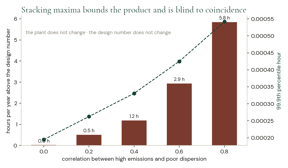
Figure 3. Exceedance frequency against the correlation between emissions and poor dispersion, with the design number and the facility held fixed.

05 · A short test of an intermittent source does not estimate a number. It fails to identify one.

The estimator is unbiased in the mean and useless in every instance, which are not the same defect as noise.

A three-hour annual stack test observes 3.4 parts in ten thousand of the year. The corpus has already computed the duty cycle of quarterly leak monitoring at 1.3 parts in a million. The usual reading of these numbers is that the resulting estimate is noisy. That reading is too kind, and simulation shows why.

Take a source that emits a steady base plus occasional bursts, and vary how much of the annual mass lives in the bursts. Test for three hours at a uniformly random moment and scale the observation up to a year. For a steady source the estimate is exact. For a source with 80 percent of its mass in twelve six-hour events, the median test reports 20 percent of the truth and 98.8 percent of tests report at most half of it, because the typical test lands in no event at all; the mean of the estimator is still 1.0, rescued entirely by the rare test that falls inside a burst and then overstates by as much as a factor of 195. Put 95 percent of the mass into four three-hour events and the median test reports 5 percent of the truth, and the luckiest test in two hundred thousand reports 693 times the truth.

This is a different failure from measurement error, and it has a name in estimation: the quantity is not identified by the design. No refinement of the instrument, no tightening of the method, no additional care in the laboratory changes it, because the information about the missing mass was never in the sample. The only fixes are to observe for longer or to observe continuously. And it lands hardest exactly where the record says the mass is: the heavy-tailed emitter, the super-emitter, the abnormal-mode event. The corpus’s own evidence dossier records that a small percentage of sources contribute the majority of point-source methane. A design that reliably misses the tail is not a conservative design.

Three-hour test, estimate as a multiple of the true annual mass (200,000 uniformly placed tests). Steady source: median 1.00, max 1.00. Half the mass in 12 events of 6 h: median 0.50, mean 1.00, max 164. 80% in 12 events of 6 h: median 0.20, mean 1.00, max 195, with 98.8% of tests reporting at most half the truth. 95% in 4 events of 3 h: median 0.05, mean 1.02, max 693, 99.7% reporting at most half. Observational duty cycle: 3-hour annual test 3.4e-4; quarterly Method 21 1.3e-6; CEMS at 95% availability 0.95.

VERIFIED: SIMULATION

06 · Every frozen model has a half-life.

The world drifts. A model calibrated once decays at a rate nobody measures, and a permit term is a bet on that rate.

A model has parameters: an emission factor, a control efficiency, a decay rate, a roughness, a rating curve. They are calibrated once, from a campaign, and then frozen for the life of the permit. Meanwhile the plant fouls its scrubber, changes feedstock, replaces a burner; the river’s channel shifts; the catchment gains pavement. Treat that drift as a random walk of step variance q per hour, and the arithmetic is unforgiving. The frozen model’s error variance is R/n + q·t, where R is the noise of a single measurement and n the number taken during calibration. It grows without bound. A model that keeps assimilating has an error variance that stops growing, at the Kalman steady state, at a level set by how often it looks rather than by how long it has run.

The crossing point is the useful object. The frozen model’s error reaches the noise of a single fresh measurement at t = R/q. Past that moment, one new reading is a better estimate of the parameter than the entire calibrated model. Call that the model’s half-life. In the simulated ensemble it arrives at 1.1 years for a moderate drift rate, and the assimilating model sits flat at a tenth of the observation noise throughout.

What makes this more than an analogy is that the half-life is a property of the world, not of the model’s quality. A better calibration campaign lowers the starting error and does not change the slope. Only a slower-drifting plant lengthens the half-life. So a five-year permit term is a bet that the facility’s drift rate keeps its model’s half-life above five years, and nobody measures drift rates, so nobody knows whether the bet is being won. Continuous monitoring is often sold as a way of catching violations. Its deeper function is that it is the only way to find out how fast your own model is decaying.

Ensemble of 400 worlds, drift q = 1e-4 per hour, observation noise R = 1.0, calibrated once from 24 hours. Frozen RMSE: 0.202 at 1 day, 0.334 at 1 month, 0.981 at 1 year, 1.762 at 3.4 years (theory √(R/n + q·t): 0.210 / 0.337 / 0.958 / 1.744). Assimilating RMSE: flat at 0.095–0.103 throughout; Kalman steady state 0.0100 → RMSE 0.100. Half-life R/q: q = 1e-3 → 0.11 yr; 1e-4 → 1.14 yr; 1e-5 → 11.4 yr; 1e-6 → 114 yr.

VERIFIED: SIMULATION TRACKS THEORY

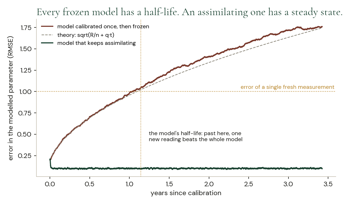
Figure 4. Error in a modelled parameter over time, for a model calibrated once and for one that keeps assimilating. The frozen model’s error grows as the square root of elapsed time; the assimilating model’s does not grow at all.

07 · The value of a model is the age of its inputs.

Refresh at the world’s tempo and most of the available knowledge appears at once. Refresh far slower and you are not looking at all.

Ask how often a picture has to be retaken to be worth having. Let the world be a process that turns over in about three days, which is the synoptic weather scale that governs dispersion; let a model be given observations at some interval and let it use them optimally, propagating between them and decaying toward climatology as its information ages. Never looking gives an error of 1.00 by construction. Hourly assimilation gives 0.26. Daily, 0.62. Weekly, 0.90. Monthly, 0.97. Quarterly, 0.98. Once every five years, 0.99.

The shape is what matters. The curve is steep exactly where the regulatory cadences sit and flat on both sides of them. Refreshing monthly a model of a world that turns over in three days is statistically almost indistinguishable from never looking, and the five-year refresh of a permit sits on the same flat shelf as never looking. That is not rhetoric: it is the same 1 percent of skill.

Read the other direction, it is the most encouraging result here. Nothing exotic is required to capture most of the available knowledge. Getting from monthly to daily is worth more than everything from daily to instantaneous. This is the same finding that the loop work reached from the detection side, and it puts a ceiling on the ambition as well as a floor: refresh at the world’s own tempo, and stop. The physics of the model is not what was limiting. The age of its inputs was.

OU world, correlation time 72 h, unit climatological variance, observation noise variance 0.25, optimal filtering. RMSE about the present state: hourly 0.26; 6-hourly 0.43; daily 0.62; weekly 0.90; monthly 0.97; quarterly 0.98; annual 0.99; every 5 years 0.99. Never looking = 1.00.

VERIFIED: SIMULATION

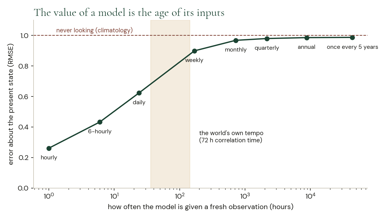
Figure 5. How much a model knows about the present state, against how often it is given a fresh observation. Regulatory cadences sit on the flat shelf at the right.

08 · The conservatism was never free. It was paid in production, every hour, for fifty years.

A static number is not a safety margin. It is the price of not knowing which hour it is.

This is the argument in the form an operator will care about, and it is the same argument. A static permit must choose one emission rate that is acceptable on the worst hour it might encounter. A live envelope may hold the same receptor limit and the same exceedance budget, and modulate the rate against the dispersion actually available in the hour.

Hold the risk exactly constant and compare the mass. Against a lognormal hourly dispersion factor and an allowed exceedance of one hour in ten thousand, a plant that can modulate by 1.5 to 1 may emit 1.36 times the static permit; by 2 to 1, 1.78 times; by 3 to 1, 2.64 times; by 5 to 1, 4.38 times. With unconstrained modulation, 9.7 times. Same limit at the receptor. Same probability of exceeding it. The only difference is that the emission is placed in the hours that can carry it.

That factor is the size of the tax the snapshot has been levying, and it explains why this transition will not need a regulator to force it. The corpus’s own commercial finding fits here: a sensor without an actuator is the worst position, multiplying records while reducing violation-days only modestly. The value is not in the measurement. It is in the pairing of a measurement with a response that is authorized in advance, which is the same design the loop work reached from the control side. The number above is what the pairing is worth, and it is a production number, not a compliance number.

One honest caution. Trading a crude static margin for a tight dynamic envelope raises exposure to model error in the tail, and where the boundary is irreversible that trade can increase the probability of crossing it even while every measured metric improves. The headroom is real. It should be spent where errors are correctable and left unspent where they are not.

Same receptor limit, same exceedance budget (1e-4 of hours), lognormal hourly dispersion, sigma_ln = 0.7. Permitted mass relative to the static permit: turndown 1.5:1 → 1.36×; 2:1 → 1.78×; 3:1 → 2.64×; 5:1 → 4.38×; unlimited → 9.68×.

VERIFIED: SIMULATION · ESTIMATE: REAL TURNDOWN LIMITS VARY BY PROCESS

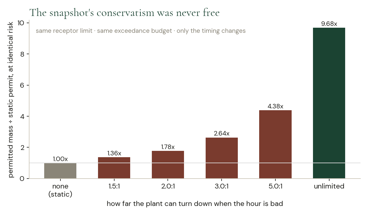
Bar chart headed “The snapshot’s conservatism was never free,” annotated “same receptor limit · same exceedance budget · only the timing changes.” Permitted mass relative to the static permit rises from 1.00× with no turndown to 1.36× at 1.5:1, 1.78× at 2:1, 2.64× at 3:1, 4.38× at 5:1 and 9.68× with unlimited modulation.

Figure 6. How much more mass the same receptor limit permits, at identical risk, as a function of how far the plant can turn down when the hour is bad.

09 · It has already started, and it started in 2003.

The transition is not a forecast. It is a practice with two decades of precedent and a cost curve that has just made it general.

The strongest evidence that the snapshot era is closing is that the replacement already runs. In 2003 the USGS published the design for the Pee Dee, Waccamaw, and Atlantic Intracoastal Waterway system near Myrtle Beach, South Carolina. A TMDL for ammonia and biochemical oxygen demand mandated a 60 percent reduction in point-source loading, and a variable loading scheme was developed so that dischargers could use the additional assimilative capacity available at higher streamflows while still meeting the TMDL; a real-time network was established across the watershed collecting continuous streamflow, water level, dissolved oxygen, temperature, and specific conductance, dynamic models were calibrated to the system’s tidal behaviour, and the scheme set total loadings for three streamflow levels. That is a permit written as a function of a measured state, in the United States, twenty-three years ago, under existing law.

Two things have changed since. The first is the cost of a model run. Aurora, a foundation model trained on more than a million hours of geophysical data, outperforms operational forecasts for air quality, ocean waves, cyclone tracks, and high-resolution weather. On air quality it matches or beats the operational CAMS system on 74 percent of targets across lead times, and on 89 percent of variables at a three-day lead. It beats the operational IFS on 92 percent of targets while running roughly 5,000 times faster. A model run stops being a project and becomes an operation you can afford to repeat every hour. (The corpus’s working research note cites a figure of 100,000 times faster than CAMS for air pollution; the primary source supports about 5,000 times faster than IFS, and that is the number to use.)

The second is that the control side is being built. A published integrated real-time control study of river water quality found operational cost savings rising from 9 to 11 percent by moving from seasonal operation to a 15-minute control step, by exploiting dynamic dilution capacity, and observed directly that traditional static year-round numeric effluent limits would be prone to violation under such control because effluent quality fluctuates. That sentence is the whole transition in miniature: the physics rewards the dynamic operation, and the static grammar of the permit is what stands in the way. Industrial sites in Europe are already coupling hourly weather forecasts with site emission forecasts to plan activity two to three days ahead and to activate emission reduction only when the forecast requires it, precisely because those actions cost tens of thousands of euros a day and should not be taken blindly.

And the legal vessel exists. This corpus has already located it: Compliance Assurance Monitoring under Part 64 requires permits to specify monitored indicators, ranges, and corrective duties, and has since 1997. What is wrong with it is not its form but its contents: the indicators are parametric surrogates, the ranges are frozen numbers set once at issuance, and the corrective duty runs on a human clock. The reform is to put a live function where the frozen range sits.

Verified. Myrtle Beach hydrograph-controlled release scheme: USGS, Environmental Monitoring and Assessment, 2003; 60% mandated load reduction; loadings set for three streamflow levels; BRANCH/BLTM dynamic models; continuous real-time network. Aurora: Nature 641:1180–1187 (2025); CAMS 74% across lead times, 89% at 3 days; ~5,000× faster than IFS. Integrated real-time control: Environmental Science & Technology 51(17):9876 (2017), 9→11% cost saving at a 15-minute step.

VERIFIED: PRIMARY SOURCES · CORRECTED: CORPUS 100,000× FIGURE

What replaces it: a model that never stops running.

The output changes from a number to a function. The snapshot’s product is a scalar: pounds per hour, milligrams per litre, for five years. The replacement’s product is a rule evaluated continuously against the measured state of the receiving environment. This corpus has already argued that the rule language, not any particular rule, is the jump, and that the consequence which fires from it must sit where the record shows consequences surviving. Sections 02 through 04 say why the scalar was never adequate: it cannot carry a curvature, a sampling error, or a correlation, and all three are properties of the world rather than deficiencies of the modeller.

The model’s job changes from prediction to state estimation. Sections 06 and 07 are one finding stated twice. A model’s error about the world is governed by the age of its inputs and by the drift of the thing it describes, not by the sophistication of its physics. A model that assimilates has a steady state; a model that is frozen has a half-life. The engineering question stops being “is the model right” and becomes “when did it last look, and how fast is the plant drifting”, and both of those are measurable.

The margin changes from a constant to a variable, and gets spent. Section 08 gives the size of the prize and the caution that goes with it. A static number is the price of not knowing which hour it is. Knowing which hour it is returns most of that price, and it should be returned only where the errors are correctable.

And the snapshot does not disappear. It moves. Someone still has to choose the receptor, the analyte, the goal, and the allocation rule, in advance, in public, and those choices are ex ante and always will be. Monitoring does not escape the ex ante problem; it inherits it. What ends is the practice of freezing a prediction about a moving system and calling it a fact. The picture becomes a feed. The permit stops being a photograph of the plant and becomes the plant’s own reflex.

We never had a modelling problem. We had a shutter speed, and we mistook the photograph for the world.

Method

Every experiment was written and run for this piece in Python (NumPy, SciPy); scripts and run logs accompany it.

Plume. Gaussian plume, 50 m effective stack height, Briggs open-country dispersion coefficients, maximum ground-level concentration taken over downwind distance for each stability class; stability frequencies are a plausible open-country mix and are illustrative, not an observed record. This is a screening calculation, not AERMOD; only the ratios are meant to be quoted.

02. Jensen’s inequality with the exact Weibull identity; the truncated cases use rejection sampling, 600,000 draws. 03. Order statistics of an exponential tail, theoretical SD √(Σ_{j≥k} 1/j²) checked against 1,500 simulated five-year records; permit-unit example assumes a tail scale of 15% of the design value and is illustrative. 04. Gaussian copula between emission rate and the dispersion factor, with the plume’s own marginal preserved by rank mapping; 400,000 hours per correlation. 05. 200,000 uniformly placed three-hour tests against a base-plus-bursts source. 06. Random-walk parameter with Kalman filtering, ensemble of 400 worlds, 30,000 hours. 07. OU state with Kalman propagation between observations at each interval, 400,000 hours. 08. Lognormal hourly dispersion factor, bisection on the nominal rate until the exceedance budget binds exactly, with a turndown floor.

What was not done, and what to distrust. No result here was checked against an observed meteorological record or a real facility; the synthetic met is a stand-in and the absolute magnitudes carry no weight. The correlation magnitudes in section 04 are asserted as plausible, not measured; identifying the actual correlation between emissions and dispersion at a real plant is the obvious next experiment and would be worth doing on TCEQ event data. The drift rates in section 06 are illustrative because, as the section says, nobody publishes drift rates. The headroom in section 08 assumes the plant can modulate on the timescale of the dispersion, which is true of some processes and false of others. Standard results relied on: Jensen’s inequality; the Fisher–Tippett–Gnedenko theorem and the Gumbel domain for the order-statistic argument; the Kalman filter’s steady state; Briggs (1973) dispersion coefficients. Verified external sources are cited inline in section 09.